Neural Scaling LawPredicting AI gains before training
A neural scaling law is a mathematical relationship showing how an AI model's error rate drops predictably as you increase its size, training data, or computing power. Instead of guessing how a larger network will perform, engineers use these power-law curves to forecast performance before spending millions on a big training run. The trade-off is steep: every fixed improvement in accuracy requires multiplying the total resources.
By the edgi team We find the most surprising true thing about an idea and build a 60-second lesson around it.
To evaluate a large language model, give it text it has not seen. At each next token, it assigns probabilities to possible continuations. The loss gets lower when the model gives more probability to the token that actually follows. In 2020, researchers plotted loss against training compute.
On logarithmic axes, the measurements followed a near-straight line across more than seven orders of magnitude. That pattern is a power law. Multiply compute by ten and loss falls by a predictable fraction over the measured range.
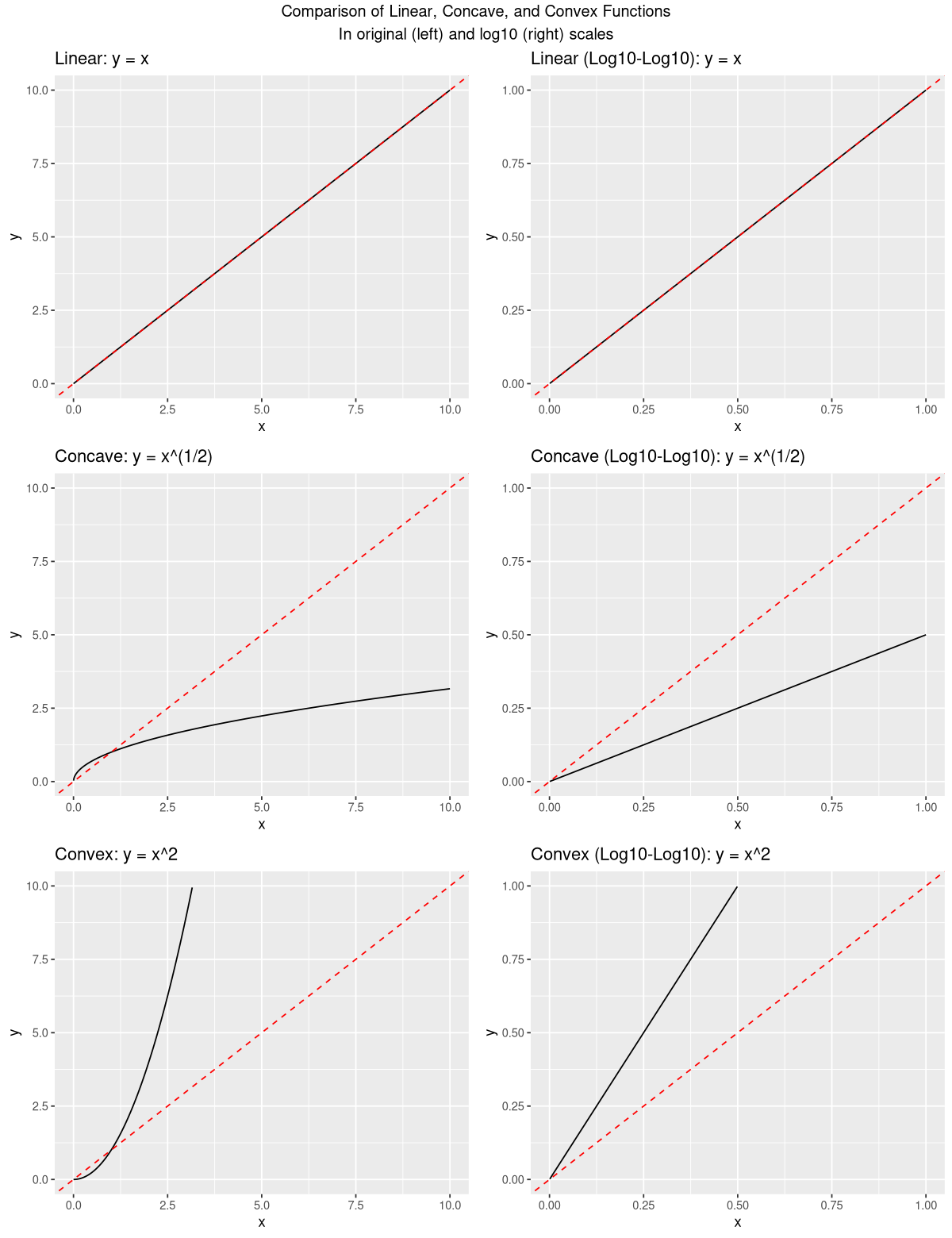
Comparison of linear, concave, and convex functions plotted on linear scales (left column) and log-log scales (right column). Talgalili, CC BY-SA 4.0, via Wikimedia Commons
Estimating the big run
A fitted power law lets a lab estimate loss at a scale it has not yet trained. Before training GPT-4, OpenAI fit scaling laws on much smaller runs and used them to predict the larger model's final loss.
That makes the cost and expected loss of a large run easier to plan before the run is complete. The tradeoff remains steep: another fixed improvement in loss needs a multiple of the compute.
The shape, and the limit
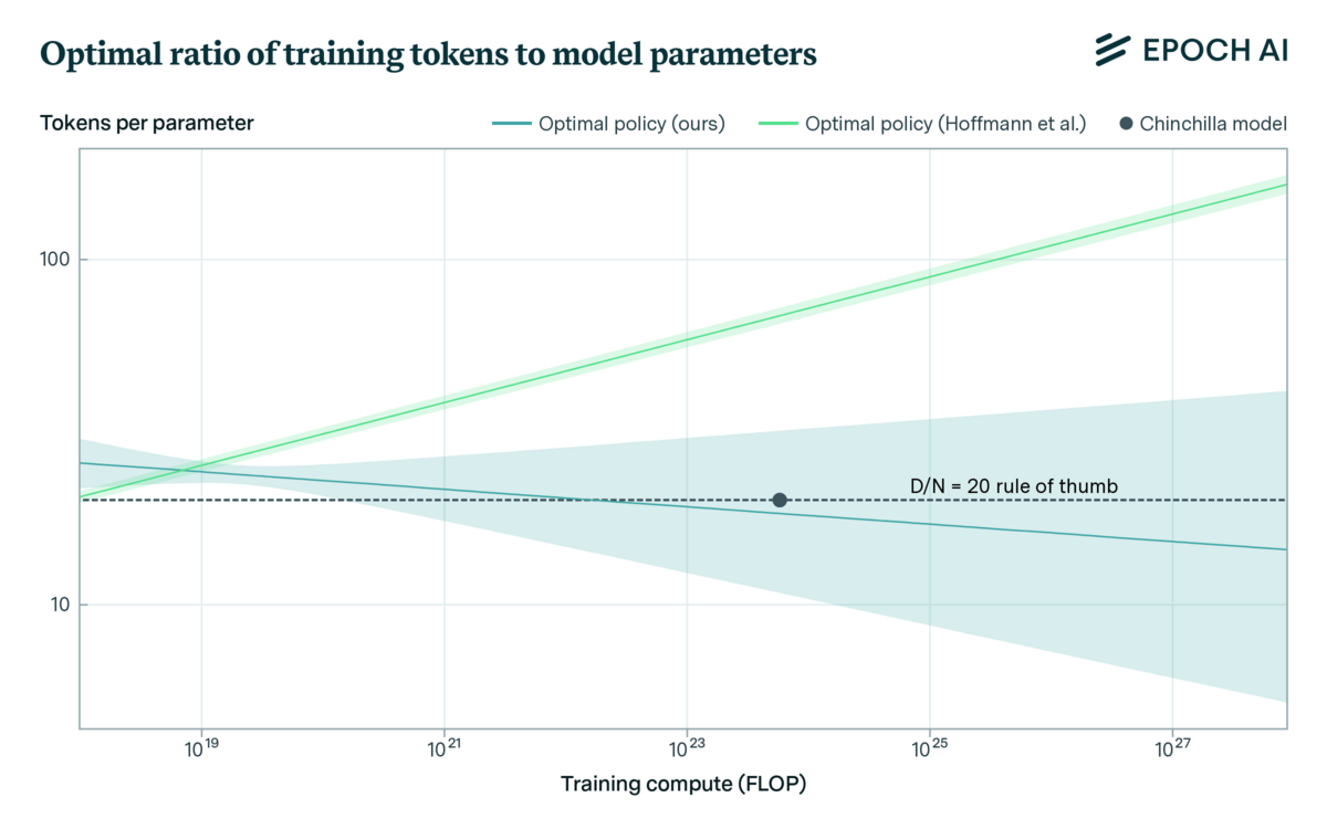
In 2022, DeepMind showed that a compute budget should balance model size with training data, not simply favor a larger model. Chinchilla used 70 billion parameters and 1.4 trillion training tokens. With the same compute budget, it outperformed the 280-billion-parameter Gopher model.
The Chinchilla result found that, for compute-optimal training in that study, doubling model size should be matched by doubling training tokens. Scaling laws predict aggregate loss well. They do not by themselves tell you which specific ability will appear at a particular size.
Graph titled "Optimal ratio of training tokens to model parameters" plots Tokens per parameter on the Y-axis (log scale) against Training compute (FLOP) on the X-axis (log scale). Epoch AI, CC BY 4.0, via Wikimedia Commons
Some aggregate capability measures can also be forecast from scaling laws. But a hard right-or-wrong score can make smooth improvement look like a sudden jump.
How do scaling laws work?
A deep learning system is defined by four core variables: parameter count (model size), dataset size, computing cost, and the resulting error rate or loss. When researchers plot error against compute on logarithmic axes, the relationship forms a straight line across multiple orders of magnitude.
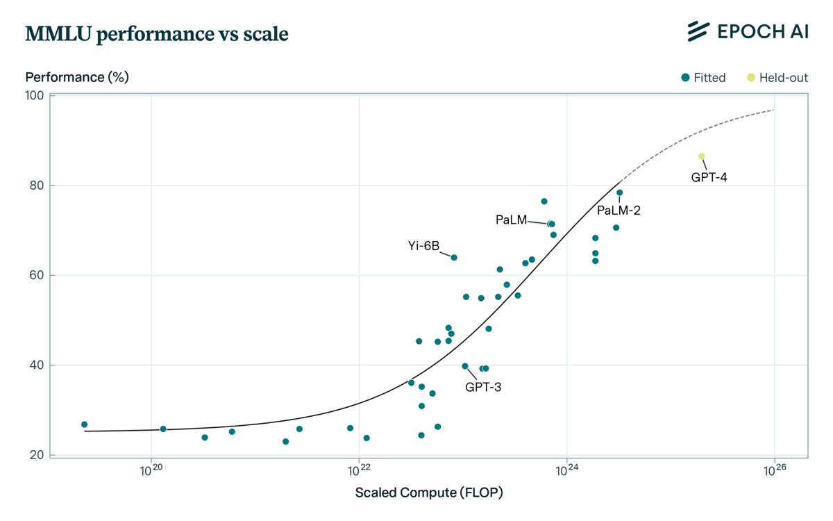
Benchmark scores bounded between zero and one follow a sigmoid curve as model scale increases. Epoch AI, CC BY 4.0, via Wikimedia Commons
Early research found that changing optimizers, regularizers, or neural network architectures alters the baseline efficiency but leaves the overall scaling exponent unchanged. Only the underlying task fundamentally alters how steeply the error curve drops as data grows.
Performance metrics bounded between zero and one, such as classification accuracy or benchmark scores, typically follow an S-shaped sigmoid curve rather than a pure power law. This sigmoid shape explains why smooth drops in loss can look like sudden jumps in capability on hard right-or-wrong tests.
Balancing model size and data
Making a neural network larger without enough data leads to wasted compute. In 2022, DeepMind trained Chinchilla with 70 billion parameters and 1.4 trillion tokens, outperforming the older 280-billion-parameter Gopher model under the exact same compute budget.
The Chinchilla results demonstrated that compute-optimal training requires doubling the training data whenever you double the parameter count. Instead of pouring all available resources into building wider models, optimal efficiency demands a strict balance between parameters and tokens.
Scaling beyond training
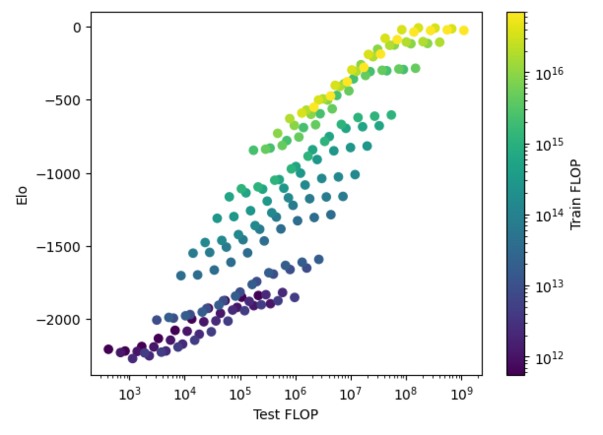
Scaling laws also apply after training ends. Systems can achieve lower error rates during deployment by scaling test-time compute, allowing the network more computing power to evaluate outputs during inference.
Game-playing AI agents gain higher Elo ratings as both training-time and test-time compute increase. Pablo Villalobos David Atkinson, CC BY 4.0, via Wikimedia Commons
Sparse architectures, such as mixture-of-experts models, modify traditional scaling math by activating only a fraction of their total parameters for any single input during inference. Standard transformer models, by contrast, use all their parameters on every run.
Test yourself
How should a fixed compute budget be allocated under neural scaling principles?
Grow model size and data in tandem. Compute-optimal training requires balancing model parameters and training tokens rather than simply inflating the model size.
What does a neural scaling law plot on logarithmic axes to reveal a power law?
Training compute against model loss. Plotting training compute against loss across logarithmic axes reveals a predictable straight-line trend known as a power law.
Under a fixed compute budget, a lab doubles model size but not training tokens. What is the risk?
The model is no longer compute-optimal. In the Chinchilla study, model size and training tokens needed to scale together for a fixed compute budget. More parameters alone need not give the best result.
Play the lesson in edgi and the card is yours. It lands on your Map next to the ideas it connects to, and turns from matte to foil to gold as you learn more around it.
How is model performance measured in scaling laws?
Performance is measured using specific error metrics, such as negative log-likelihood per token for language models, mean squared error for regression, and accuracy or F1 score for classification tasks. Competitive models are also evaluated using Elo ratings from games or head-to-head human preference tests.
Does fine-tuning follow the same scaling as pre-training?
Fine-tuning datasets are typically less than 1% the size of pre-training datasets and behave differently. In many cases, a small amount of high-quality data is sufficient for fine-tuning, and adding more data does not necessarily improve performance.